Quickstart with 10x Genomics Data

This tutorial will walk you through analyzing a real-world single-cell RNA-seq dataset using SCRIBE. For this tutorial, we will use the Jurkat cells dataset from 10x Genomics (available here). To ilustrate SCRIBE’s flexibility, we will explore several models available, starting from the basic Negative Binomial-Dirichlet Multinomial (NBDM) model where all genes are negative binomially distributed with a shared success probability \(p\) and a gene-specific \(r_g\) parameter. Later on, we will account for the cell-to-cell variation in mRNA-to-UMI conversion efficiency by explicitly modeling the mRNA capture efficiency. Finally, we will explore a different parameterization of the model to help with convergence and performance.

Setup

First, let’s import the necessary libraries and set up our directories.

import os
from jax import random
import numpy as np
import matplotlib.pyplot as plt
import seaborn as sns
import scanpy as sc  # to load the data
import scribe  # our main library
import pickle  # to save the results

# Define directories
OUTPUT_DIR = "output"
FIG_DIR = os.path.join(OUTPUT_DIR, "figures")

# Create output directory
os.makedirs(OUTPUT_DIR, exist_ok=True)
os.makedirs(FIG_DIR, exist_ok=True)

# Simple cache directory. This directory is used to store the results of the
# models for this tutorial to avoid re-running the models as we work through the
# tutorial. YOU DO NOT NEED TO DO THIS IN YOUR OWN ANALYSIS.
CACHE_DIR = "../../../CACHE"
os.makedirs(CACHE_DIR, exist_ok=True)


# Set plotting style and scanpy settings
scribe.viz.matplotlib_style()
sc.settings.verbosity = 1  # Reduce scanpy output verbosity for cleaner tutorial

Loading the Data

We will use the Jurkat cell dataset from 10x Genomics. This dataset consists of ~3,200 human Jurkat cells, a T-lymphocyte cell line. For this tutorial, we’ll use the full transcriptome to demonstrate SCRIBE’s ability to handle large-scale single-cell datasets.

Note

SCRIBE is designed to work with the entire transcriptome and can easily handle datasets with 20,000+ genes, as long as you have the right hardware. This is the recommended approach for comprehensive analysis.

# Define path to the data
data_path = os.path.abspath(
    os.path.join(
        os.path.dirname(scribe.__file__),
        # Here, put the path to the data.h5ad file in your computer.
        "../../data/10xGenomics/Jurkat_cells/data.h5ad",
    )
)

# Load the data using scanpy
adata = sc.read_h5ad(data_path)

# Extract raw counts for ``SCRIBE`` (``SCRIBE`` works with raw integer counts)
counts = adata.X.toarray()

# Define number of cells and genes
n_cells = adata.n_obs
n_genes = adata.n_vars

print(f"Count matrix data type: {counts.dtype}")
print(f"Total UMIs in dataset: {counts.sum():,.0f}")
print(f"Mean UMIs per cell: {counts.sum(axis=1).mean():.1f}")
print(f"Mean UMIs per gene: {counts.sum(axis=0).mean():.1f}")

Count matrix data type: float32
Total UMIs in dataset: 50,727,268
Mean UMIs per cell: 15570.1
Mean UMIs per gene: 1549.5

Model 1: Negative Binomial-Dirichlet Multinomial (NBDM)

The core of SCRIBE is the Negative Binomial-Dirichlet Multinomial (NBDM) model. This model is derived from first principles, where a two-state promoter model can be shown to lead to a steady-state mRNA distribution that follows a Negative Binomial (NB) distribution. The only extra-ingredient SCRIBE adds is to assume that all genes share the same success probability parameter \(p\). Biophysically, this is equivalent to assuming that all genes share the same burst size.

A key insight from this model is that if all genes share the same success probability parameter \(p\) in their NB distributions, the joint distribution of UMI counts for a cell can be factorized into two components:

1. A Negative Binomial distribution for the total number of UMIs in the cell.

2. A Dirichlet-Multinomial (DM) distribution for the relative proportions of gene counts.

This factorization allows SCRIBE to normalize gene expression levels as the math reveals a natural scheme where the gene-specific \(r_g\) parameters can be used to compute the fraction of the transcriptome that each gene occupies.

Let’s fit the basic NBDM model to our data using Stochastic Variational Inference (SVI). SVI is a type of variational inference that, although only approximately correct, is very fast and scalable, perfect for exploring large datasets quickly. For SCRIBE, all we need to specify is the number of steps to run the inference for (think of stochastic gradient descent for optimization), the batch size (how many cells to process at once for each optimization step), and a random seed for reproducibility.

# Define inference parameters
n_steps = 30_000
batch_size = 512
seed = 42

# Simple caching for NBDM model. Again, you do not need to do this in your own
# analysis if you don't want to; this is just not to re-run the model if we
# already have the results.
cache_file = os.path.join(
    CACHE_DIR, f"svi_quickstart_nbdm_standard_{n_genes}genes_{n_steps}steps.pkl"
)
if os.path.exists(cache_file):
    print(f"Loading NBDM results from {cache_file}")
    with open(cache_file, "rb") as f:
        results_nbdm = pickle.load(f)
else:
    print("Running NBDM model...")
    results_nbdm = scribe.run_scribe(
        counts=counts,  # The count matrix
        n_steps=n_steps,  # The number of steps to run the inference for
        batch_size=batch_size,  # The batch size
        seed=seed,  # The random seed
    )
    # Save the results to a file.
    with open(cache_file, "wb") as f:
        pickle.dump(results_nbdm, f)
    print(f"Saved NBDM results to {cache_file}")

Loading NBDM results from ../../../CACHE/svi_quickstart_nbdm_standard_32738genes_30000steps.pkl

Visualizing Results for NBDM

After fitting the model, we should always perform diagnostic checks to assess the model fit. We’ll look at the ELBO loss history first. What we are looking for is that the loss is decreasing over time, and that it plateaus at some point. Empirically, we have seen that anything between 25,000 and 50,000 steps is usually enough to get a good fit.

Note

Although SVI aims to maximize the ELBO, here we are looking for a decreasing loss function, this is because the actual loss function implemented in SVI is the negative ELBO, also known as the Variational Free Energy.

# Plot ELBO loss history
fig, ax = plt.subplots(figsize=(3.5, 3))
ax.plot(results_nbdm.loss_history)
ax.set_xlabel("step")
ax.set_ylabel("ELBO Loss")
ax.set_title("NBDM ELBO Loss")
plt.tight_layout()
plt.show()

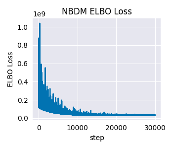
This looks good. The loss is decreasing over time, and it plateaus at some point.

After confirming that the optimization is converging, one of the most important steps in any Bayesian model (and one could argue in any statistical model) is to perform posterior predictive checks (PPCs).

PPCs are a way to check if the model is able to reproduce the key features of the observed data. The logic is straightforward:

1. Generate Synthetic Data: Use the fitted model to generate new datasets that should resemble the original data if the model is appropriate. This means that we take a sample of the posterior parameters and run them through the likelihood function to simulate a new dataset. We repeat this process multiple times to get a distribution of the predicted data.

2. Compare Distributions: Plot the distribution of observed counts alongside the distribution of model-predicted counts for the same genes. This is done by plotting the distribution of the observed counts alongside the distribution of the predicted counts for the same genes. Usually, we can plot quantiles of the predicted data to get a sense of the distribution.

3. Assess Model Fit: If the model is good, the observed data should fall within the credible intervals of the predicted data most of the time.

Important

This is not a common practice in the field of single-cell RNA-seq analysis, but we argue it should be! A simple visual inspection of the quality of the fit is vital to understand how well the model is able to capture the data.

Strategic Gene Selection for Posterior Predictive Checks

Before generating PPC samples, we need to select a subset of genes to analyze. This is because generating PPC samples is a computationally and memory intensive process. Usually, we would like to generate between 100 and 1000 samples; each sample being a full count matrix with the same number of cells and genes as the original data. You can see how this can get out of hand very quickly. Fortunately, SCRIBE’s results objects are indexable, allowing us to subset the results to only the genes we want to visualize.

Rather than randomly selecting genes for visualization, we’ll use a strategic approach that ensures we capture genes across different expression levels. This is done by calculating the median expression for each gene across all cells in the dataset, filtering out completely unexpressed genes (median = 0), sorting genes by their median expression, and selecting evenly spaced genes across the expression spectrum. However, feel free to use whatever method you prefer.

Note

We filter genes with median expression equal to 0 for visualization purposes. However, these genes were taken into account for the model fit. This is the power of the full Bayesian framework SCRIBE offers.

def select_genes_for_visualization(counts, n_genes=25):
    """
    Select a representative subset of genes for visualization based on their
    expression levels.

    This function implements a stratified sampling approach that:
        1. Calculates median expression for each gene across all cells
        2. Filters out completely unexpressed genes (median = 0)
        3. Sorts genes by their median expression
        4. Selects evenly spaced genes across the expression spectrum

    Parameters
    ----------
    counts : array-like, shape (n_cells, n_genes)
        The count matrix where rows are cells and columns are genes.
    n_genes : int, default=25
        Number of genes to select for visualization.

    Returns
    -------
    selected_idx : array
        Indices of selected genes, sorted by expression level.
    median_expr : array
        Median expression values for all genes.
    """
    # Calculate median expression across cells for each gene
    # We use median instead of mean because it's more robust to outliers
    # and better represents the typical expression level
    median_expr = np.median(counts, axis=0)

    # Find genes that are expressed in at least some cells
    # Genes with median = 0 are likely unexpressed or very lowly expressed
    expressed_idx = np.where(median_expr > 0)[0]

    # Sort expressed genes by their median expression level
    sorted_idx = expressed_idx[np.argsort(median_expr[expressed_idx])]

    # Select evenly spaced genes across the expression spectrum
    # This ensures we sample from low, medium, and high expression ranges
    spaced_indices = np.linspace(0, len(sorted_idx) - 1, num=n_genes, dtype=int)
    selected_idx = sorted_idx[spaced_indices]

    return selected_idx, median_expr


# Select genes using our strategic approach
n_genes_to_plot = 25
selected_idx, median_expr = select_genes_for_visualization(
    counts, n_genes=n_genes_to_plot
)

# Sort selected indices - this is crucial for proper indexing of results!
# This ensures correspondence between subset results and original gene indices
selected_idx = np.sort(selected_idx)

print(f"Selected {len(selected_idx)} genes for PPC analysis")
print(
    f"Expression range: {median_expr[selected_idx].min():.2f} - "
    f"{median_expr[selected_idx].max():.2f}"
)

Selected 25 genes for PPC analysis
Expression range: 0.50 - 167.00

We are now ready to generate the PPC samples. We will generate 500 samples, i.e., 500 simulated datasets with the same number of cells \(\times\) the number of genes we selected.

n_samples = (
    500  # Can use more samples now since we're only doing selected genes
)

# Subset results to selected genes before generating samples (major memory
# savings!)
results_nbdm_subset = results_nbdm[selected_idx]
# Generate the PPC samples
ppc_nbdm = results_nbdm_subset.get_ppc_samples(
    n_samples=n_samples, rng_key=random.PRNGKey(seed)
)

Now, since we will generate a plot for each selected gene, we need to calculate the optimal number of rows and columns for the plot grid. Let’s define a simple function to do this.

def calculate_subplot_grid(n_plots):
    """
    Calculate optimal subplot grid dimensions for a given number of plots.

    Tries to create a square or near-square grid that accommodates all plots.

    Parameters
    ----------
    n_plots : int
        Number of subplots needed

    Returns
    -------
    nrows, ncols : int, int
        Number of rows and columns for the subplot grid
    """
    import math

    # For perfect squares, use square grid
    sqrt_n = int(math.sqrt(n_plots))
    if sqrt_n * sqrt_n == n_plots:
        return sqrt_n, sqrt_n

    # For non-perfect squares, find the closest rectangular grid
    # that minimizes empty subplots
    for cols in range(sqrt_n, n_plots + 1):
        rows = math.ceil(n_plots / cols)
        if (
            rows * cols >= n_plots and abs(rows - cols) <= 2
        ):  # Prefer near-square
            return rows, cols

    # Fallback: use ceiling of square root
    rows = math.ceil(math.sqrt(n_plots))
    cols = math.ceil(n_plots / rows)
    return rows, cols

Posterior Predictive Check Visualization

We are ready to plot the PPCs. We will plot the credible regions for each gene as colored bands, and the observed data as a black line. We will also plot the median expression for each gene. SCRIBE provides several useful functions to generate these plots.

# Plot PPCs for selected genes with dynamic grid layout
n_genes_to_plot = len(selected_idx)
nrows, ncols = calculate_subplot_grid(n_genes_to_plot)
fig_width = max(12, ncols * 3)  # Minimum 12 inches, scale with columns
fig_height = max(8, nrows * 2.5)  # Minimum 8 inches, scale with rows

# Print the number of rows and columns for the plot grid
print(f"Creating {nrows}x{ncols} grid for {n_genes_to_plot} genes")

# Initialize the plot
fig, axes = plt.subplots(nrows, ncols, figsize=(fig_width, fig_height))
# Flatten the axes if we have more than one gene to plot
axes = axes.flatten() if n_genes_to_plot > 1 else [axes]

# Add a title to the plot
fig.suptitle(
    f"NBDM Posterior Predictive Checks ({n_genes_to_plot} genes)",
    y=0.98,
    fontsize=16,
)

# Loop over the genes to plot
for i in range(n_genes_to_plot):
    ax = axes[i]
    gene_idx = selected_idx[i]
    gene_median_expr = median_expr[gene_idx]

    print(
        f"Generating PPC for gene {gene_idx} "
        f"(median expression: {gene_median_expr:.2f})"
    )

    # Compute credible regions for this gene's predicted counts
    # Note: gene_idx is now the index within selected genes, not the original
    # dataset
    credible_regions = scribe.stats.compute_histogram_credible_regions(
        ppc_nbdm["predictive_samples"][
            :, :, i
        ],  # Use i (position in selected genes)
        credible_regions=[95, 68, 50],
    )

    # Plot the credible regions as colored bands
    scribe.viz.plot_histogram_credible_regions_stairs(
        ax, credible_regions, cmap="Blues", alpha=0.5
    )

    # Calculate and plot the observed data histogram
    bin_edges = credible_regions["bin_edges"]
    hist, _ = np.histogram(counts[:, gene_idx], bins=bin_edges, density=True)
    ax.stairs(
        hist, bin_edges, color="black", alpha=0.8, linewidth=2, label="Observed"
    )

    # Enhanced axis labels with expression information
    ax.set_xlabel(f"UMI counts")
    ax.set_ylabel("density")
    ax.set_title(
        f"{adata.var.index.values[gene_idx]}\n"
        f"(Median expr: {gene_median_expr:.1f})",
        fontsize=10,
    )
    ax.legend(fontsize=8)

    # Improve readability for low-count genes
    if gene_median_expr < 1.0:
        ax.set_xlim(0, max(10, np.percentile(counts[:, gene_idx], 95)))

# Hide empty subplots if we have more subplot positions than genes
for j in range(n_genes_to_plot, len(axes)):
    axes[j].axis("off")

plt.tight_layout()
plt.show()

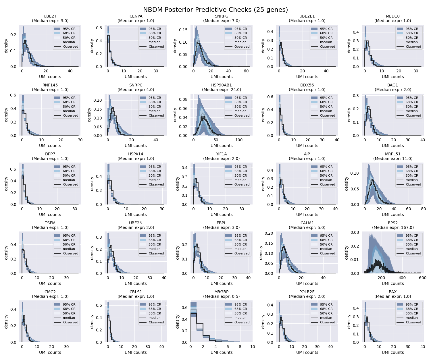
Creating 5x5 grid for 25 genes
Generating PPC for gene 2629 (median expression: 3.00)
Generating PPC for gene 3488 (median expression: 1.00)
Generating PPC for gene 3902 (median expression: 7.00)
Generating PPC for gene 5592 (median expression: 1.00)
Generating PPC for gene 8585 (median expression: 1.00)
Generating PPC for gene 9886 (median expression: 1.00)
Generating PPC for gene 10744 (median expression: 4.00)
Generating PPC for gene 10916 (median expression: 24.00)
Generating PPC for gene 12225 (median expression: 1.00)
Generating PPC for gene 15825 (median expression: 2.00)
Generating PPC for gene 16829 (median expression: 1.00)
Generating PPC for gene 17017 (median expression: 1.00)
Generating PPC for gene 19203 (median expression: 2.00)
Generating PPC for gene 19259 (median expression: 1.00)
Generating PPC for gene 20152 (median expression: 11.00)
Generating PPC for gene 20954 (median expression: 1.00)
Generating PPC for gene 21229 (median expression: 2.00)
Generating PPC for gene 22057 (median expression: 3.00)
Generating PPC for gene 23206 (median expression: 5.00)
Generating PPC for gene 24673 (median expression: 167.00)
Generating PPC for gene 25837 (median expression: 1.00)
Generating PPC for gene 28675 (median expression: 1.00)
Generating PPC for gene 29321 (median expression: 0.50)
Generating PPC for gene 29443 (median expression: 2.00)
Generating PPC for gene 30931 (median expression: 1.00)

We can see that the fit is already pretty good. Most of the observed counts fall within the colored regions, meaning that the inferred parameters are able to capture the observed data. However, we can improve the fit by using a more sophisticated model.

Model 2: NBDM with Variable Capture Probability (NBVCP)

The basic NBDM model assumes that the capture efficiency—the probability of an mRNA molecule being captured and sequenced as a UMI—is constant for all cells. However, this is often not true in practice due to technical variations. To demonstrate this, let’s plot the distribution of total UMI counts for each cell.

# Initialize figure
fig, ax = plt.subplots(figsize=(3.5, 3))
sns.histplot(counts.sum(axis=1), bins=100, ax=ax)
ax.set_xlabel("total UMI counts")
ax.set_ylabel("count")
ax.set_title("Distribution of Total UMI Counts")
plt.tight_layout()
plt.show()

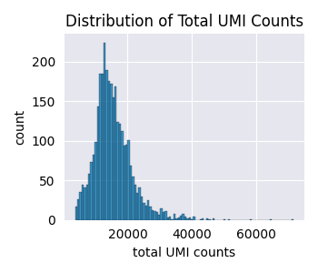
These cells were already filtered for quality and still we have cells with \(\approx\) 5,000 UMIs vs cells with \(\approx\) 40,000 UMIs. This is unlikely to be due to biological differences, but rather to technical differences in the capture efficiency.

SCRIBE can account for this by using a Variable Capture Probability (VCP) model. As mentioned earlier, in the derivation of the NBDM model, we assumed all mRNA counts to be negative-binomially distributed. However, what we observe in an experiment are not the mRNA counts, but the UMIs. The simplest way to account for this conversion is to assume that each mRNA molecule in cell \(c\) has a probability \(\nu^{(c)}\) of being captured and sequenced as a UMI. We can show that after accounting for this effect, the resulting UMI counts distribution is also negative-binomially distributed. However, the parameter \(p\) is modified in a non-linear was as

\[\hat{p}^{(c)} = \frac{p}{\nu^{(c)} + p (1 - \nu^{(c)})}.\]

In this model, the capture efficiency \(\nu^{(c)}\) is a cell-specific latent variable that is inferred from the data. This allows the model to distinguish between biological zeros (genes not expressed) and technical zeros (genes expressed but not detected).

Important

Note that this is very different from the conventional approach of assuming a zero-inflated negative binomial distribution (which SCRIBE also supports). Zero-inflation in that sense is a per-gene parameter, while our approach is a per-cell parameter. Although it might be possible that there is a per-gene capture efficiency across all cells, we find it much more likely that the tehcnical variation comes from processing each cell separately.

Let’s fit the NBVCP model. The beauty of the API is that we can fit this variant by simply passing the variable_capture=True flag.

# Simple caching for NBVCP model
cache_file = os.path.join(
    CACHE_DIR,
    f"svi_quickstart_nbvcp_standard_{n_genes}genes_{n_steps}steps.pkl",
)
if os.path.exists(cache_file):
    print(f"Loading NBVCP results from {cache_file}")
    with open(cache_file, "rb") as f:
        results_vcp = pickle.load(f)
else:
    print("Running NBVCP model...")
    results_vcp = scribe.run_scribe(
        counts=counts,
        variable_capture=True,  # this is the only difference from the NBDM model
        n_steps=n_steps,
        batch_size=batch_size,
        seed=seed,
    )
    with open(cache_file, "wb") as f:
        pickle.dump(results_vcp, f)
    print(f"Saved NBVCP results to {cache_file}")

Loading NBVCP results from ../../../CACHE/svi_quickstart_nbvcp_standard_32738genes_30000steps.pkl

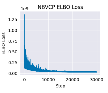
Visualizing Results for NBVCP

Now, let’s look at the diagnostics for the NBVCP model.

# Plot ELBO loss history
fig, ax = plt.subplots(figsize=(3.5, 3))
ax.plot(results_vcp.loss_history)
ax.set_xlabel("Step")
ax.set_ylabel("ELBO Loss")
ax.set_title("NBVCP ELBO Loss")
plt.tight_layout()
plt.show()

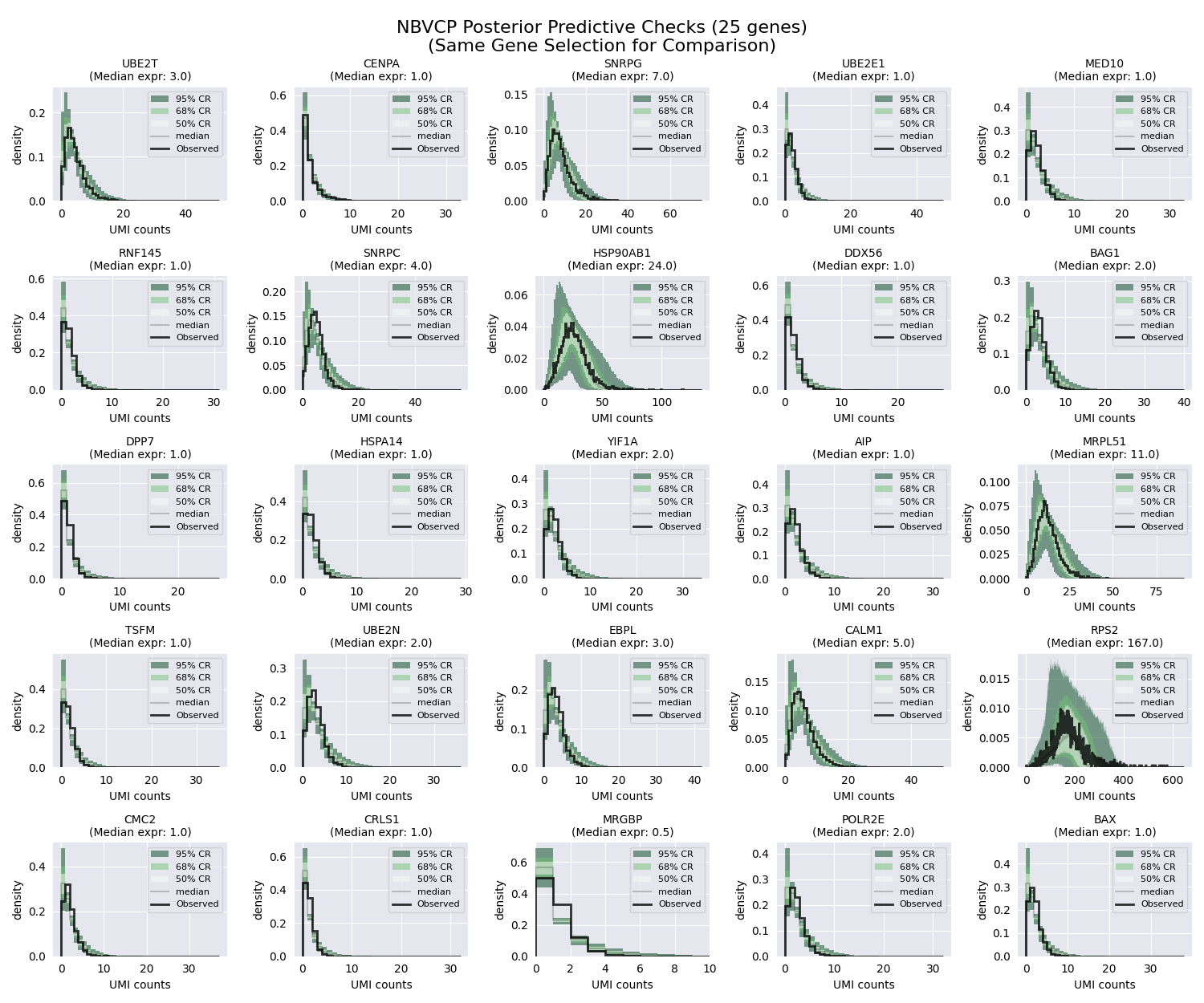
As before, we can visualize the posterior predictive checks for the NBVCP model. The unified API makes it straightforward to do so by following the same steps as before.

# Generate PPC samples for the NBVCP model (using same gene subset)
results_vcp_subset = results_vcp[selected_idx]
ppc_vcp = results_vcp_subset.get_ppc_samples(
    n_samples=n_samples, rng_key=random.PRNGKey(seed)
)

# Plot PPCs using the same strategically selected genes for fair comparison
fig, axes = plt.subplots(nrows, ncols, figsize=(fig_width, fig_height))
axes = axes.flatten() if n_genes_to_plot > 1 else [axes]
fig.suptitle(
    f"NBVCP Posterior Predictive Checks ({n_genes_to_plot} genes)\n"
    f"(Same Gene Selection for Comparison)",
    y=0.98,
    fontsize=16,
)

for i in range(n_genes_to_plot):
    ax = axes[i]
    gene_idx = selected_idx[i]
    gene_median_expr = median_expr[gene_idx]

    print(
        f"Generating NBVCP PPC for gene {gene_idx} "
        f"(median expression: {gene_median_expr:.2f})"
    )

    # Compute credible regions for this gene's predicted counts
    credible_regions = scribe.stats.compute_histogram_credible_regions(
        ppc_vcp["predictive_samples"][
            :, :, i
        ],  # Use i (position in selected genes)
        credible_regions=[95, 68, 50],
    )

    # Plot the credible regions using green colormap to distinguish from NBDM
    scribe.viz.plot_histogram_credible_regions_stairs(
        ax, credible_regions, cmap="Greens", alpha=0.5
    )

    # Calculate and plot the observed data histogram
    bin_edges = credible_regions["bin_edges"]
    hist, _ = np.histogram(counts[:, gene_idx], bins=bin_edges, density=True)
    ax.stairs(
        hist, bin_edges, color="black", alpha=0.8, linewidth=2, label="Observed"
    )

    # Enhanced axis labels with expression information
    ax.set_xlabel(f"UMI counts")
    ax.set_ylabel("density")
    ax.set_title(
        f"{adata.var.index.values[gene_idx]}\n"
        f"(Median expr: {gene_median_expr:.1f})",
        fontsize=10,
    )
    ax.legend(fontsize=8)

    # Improve readability for low-count genes
    if gene_median_expr < 1.0:
        ax.set_xlim(0, max(10, np.percentile(counts[:, gene_idx], 95)))

# Hide empty subplots if we have more subplot positions than genes
for j in range(n_genes_to_plot, len(axes)):
    axes[j].axis("off")

plt.tight_layout()
plt.show()

Generating NBVCP PPC for gene 2629 (median expression: 3.00)
Generating NBVCP PPC for gene 3488 (median expression: 1.00)
Generating NBVCP PPC for gene 3902 (median expression: 7.00)
Generating NBVCP PPC for gene 5592 (median expression: 1.00)
Generating NBVCP PPC for gene 8585 (median expression: 1.00)
Generating NBVCP PPC for gene 9886 (median expression: 1.00)
Generating NBVCP PPC for gene 10744 (median expression: 4.00)
Generating NBVCP PPC for gene 10916 (median expression: 24.00)
Generating NBVCP PPC for gene 12225 (median expression: 1.00)
Generating NBVCP PPC for gene 15825 (median expression: 2.00)
Generating NBVCP PPC for gene 16829 (median expression: 1.00)
Generating NBVCP PPC for gene 17017 (median expression: 1.00)
Generating NBVCP PPC for gene 19203 (median expression: 2.00)
Generating NBVCP PPC for gene 19259 (median expression: 1.00)
Generating NBVCP PPC for gene 20152 (median expression: 11.00)
Generating NBVCP PPC for gene 20954 (median expression: 1.00)
Generating NBVCP PPC for gene 21229 (median expression: 2.00)
Generating NBVCP PPC for gene 22057 (median expression: 3.00)
Generating NBVCP PPC for gene 23206 (median expression: 5.00)
Generating NBVCP PPC for gene 24673 (median expression: 167.00)
Generating NBVCP PPC for gene 25837 (median expression: 1.00)
Generating NBVCP PPC for gene 28675 (median expression: 1.00)
Generating NBVCP PPC for gene 29321 (median expression: 0.50)
Generating NBVCP PPC for gene 29443 (median expression: 2.00)
Generating NBVCP PPC for gene 30931 (median expression: 1.00)

For this particular dataset, the difference between the NBDM and NBVCP models is not very pronounced. However, in general, we recommend using the NBVCP model when there is evidence of technical variation in the capture efficiency.

Moreover, even though the data falls within the colored regions, there also seems to be “unnecessary” uncertainty. Take for example the HSP90AB1 gene (second row, third column). Even though the data falls within the colored regions, these regions seem to be unnecessarily wide. The reason for this is subtle but important: When performing SVI, we use what is called a “mean-field” approximaiton. This means that we fit each parameter independently, ignoring all possible correlations between parameters. This allows us to use the power of modern gradient-based optimizers to find the optimal parameters. However, this also bring an issue when working with the negative binomial distribution, where the \(r\) and \(p\) parameters trade-off with each other—meaning that increasing one parameter while decreasing the other results in a distribution with a very similar shape.

To address this issue, SCRIBE comes with two other parameterizations of the same base NBDM model:

• the linked parameterization, in which we fit the same \(p\) parameter, but instead of fitting the \(r\) parameter, we fit the distribution mean \(\mu\) parameter. We then can recover the \(r\) parameter as \(r = \mu * (1 - p) / p\).

• the odds-ratio parameterization, in which we fit the so-called odds-ratio \(\phi = (1 - p) / p\) parameter, and the \(\mu\) parameter. We then can recover the \(r\) parameter as \(r = \mu * \phi\).

Changing between parameterizations is as simple as passing the appropriate parameterization flag to the run_scribe function. Let’s fit the NBVCP model with the odds-ratio parameterization.

Model 3: Odds-Ratio Parameterization

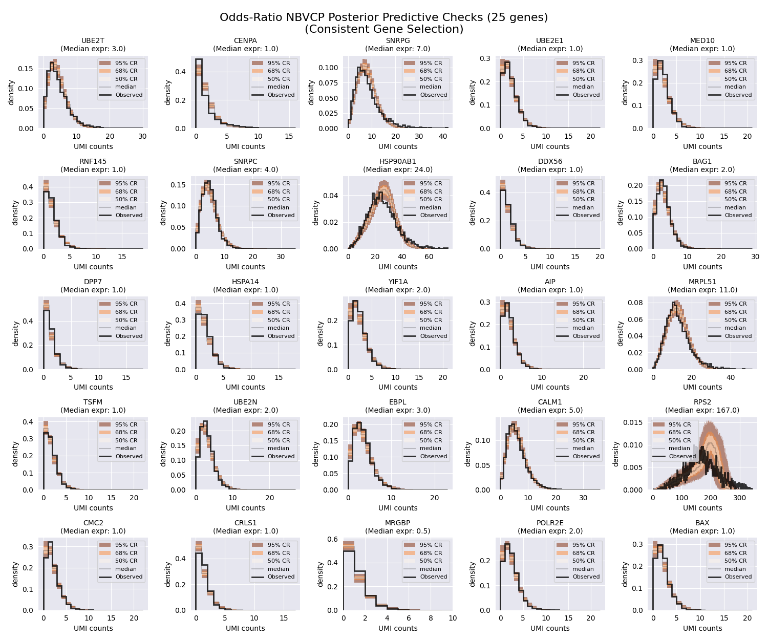
This reparameterization can lead to more stable and efficient inference, especially when the success probability p is very close to 0 or 1. Moreover, because of the mean-field approximation done for stochastic variational inference, this parameterization captures the known correlation between the r and p parameters by fitting the mean mu instead of the dispersion r. This results in much better posterior predictive checks.

Let’s fit the NBVCP model with the odds-ratio parameterization. Again, we can do this by simply passing the parameterization=”odds_ratio” flag.

# Simple caching for Odds-Ratio NBVCP model
cache_file = os.path.join(
    CACHE_DIR,
    f"svi_quickstart_nbvcp_odds-ratio_{n_genes}genes_{n_steps}steps.pkl",
)
if os.path.exists(cache_file):
    print(f"Loading Odds-Ratio NBVCP results from {cache_file}")
    with open(cache_file, "rb") as f:
        results_or = pickle.load(f)
else:
    print("Running Odds-Ratio NBVCP model...")
    results_or = scribe.run_scribe(
        counts=counts,
        variable_capture=True,
        parameterization="odds_ratio",
        n_steps=n_steps,
        batch_size=batch_size,
        seed=seed,
    )
    with open(cache_file, "wb") as f:
        pickle.dump(results_or, f)
    print(f"Saved Odds-Ratio NBVCP results to {cache_file}")

Loading Odds-Ratio NBVCP results from ../../../CACHE/svi_quickstart_nbvcp_odds-ratio_32738genes_30000steps.pkl

Visualizing Results for Odds-Ratio Model

Finally, let’s check the diagnostics for the odds-ratio model.

# Plot ELBO loss history
fig, ax = plt.subplots(figsize=(3.5, 3))
ax.plot(results_or.loss_history)
ax.set_xlabel("Step")
ax.set_ylabel("ELBO Loss")
ax.set_title("Odds-Ratio NBVCP ELBO Loss")
plt.tight_layout()
plt.show()

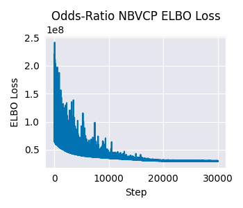
And the PPCs.

# Generate PPC samples for the odds-ratio model (using same gene subset)
results_or_subset = results_or[selected_idx]
ppc_or = results_or_subset.get_ppc_samples(
    n_samples=n_samples, rng_key=random.PRNGKey(seed)
)

# Plot PPCs using the same strategically selected genes for consistent comparison
fig, axes = plt.subplots(nrows, ncols, figsize=(fig_width, fig_height))
axes = axes.flatten() if n_genes_to_plot > 1 else [axes]
fig.suptitle(
    f"Odds-Ratio NBVCP Posterior Predictive Checks ({n_genes_to_plot} genes)\n"
    f"(Consistent Gene Selection)",
    y=0.98,
    fontsize=16,
)

for i in range(n_genes_to_plot):
    ax = axes[i]
    gene_idx = selected_idx[i]
    gene_median_expr = median_expr[gene_idx]

    print(
        f"Generating Odds-Ratio PPC for gene {gene_idx} "
        f"(median expression: {gene_median_expr:.2f})"
    )

    # Compute credible regions for this gene's predicted counts
    credible_regions = scribe.stats.compute_histogram_credible_regions(
        ppc_or["predictive_samples"][
            :, :, i
        ],  # Use i (position in selected genes)
        credible_regions=[95, 68, 50],
    )

    # Plot the credible regions using orange colormap to distinguish from other
    # models
    scribe.viz.plot_histogram_credible_regions_stairs(
        ax, credible_regions, cmap="Oranges", alpha=0.5
    )

    # Calculate and plot the observed data histogram
    bin_edges = credible_regions["bin_edges"]
    hist, _ = np.histogram(counts[:, gene_idx], bins=bin_edges, density=True)
    ax.stairs(
        hist, bin_edges, color="black", alpha=0.8, linewidth=2, label="Observed"
    )

    # Enhanced axis labels with expression information
    ax.set_xlabel(f"UMI counts")
    ax.set_ylabel("density")
    ax.set_title(
        f"{adata.var.index.values[gene_idx]}\n"
        f"(Median expr: {gene_median_expr:.1f})",
        fontsize=10,
    )
    ax.legend(fontsize=8)

    # Improve readability for low-count genes
    if gene_median_expr < 1.0:
        ax.set_xlim(0, max(10, np.percentile(counts[:, gene_idx], 95)))

# Hide empty subplots if we have more subplot positions than genes
for j in range(n_genes_to_plot, len(axes)):
    axes[j].axis("off")

plt.tight_layout()
plt.show()

Generating Odds-Ratio PPC for gene 2629 (median expression: 3.00)
Generating Odds-Ratio PPC for gene 3488 (median expression: 1.00)
Generating Odds-Ratio PPC for gene 3902 (median expression: 7.00)
Generating Odds-Ratio PPC for gene 5592 (median expression: 1.00)
Generating Odds-Ratio PPC for gene 8585 (median expression: 1.00)
Generating Odds-Ratio PPC for gene 9886 (median expression: 1.00)
Generating Odds-Ratio PPC for gene 10744 (median expression: 4.00)
Generating Odds-Ratio PPC for gene 10916 (median expression: 24.00)
Generating Odds-Ratio PPC for gene 12225 (median expression: 1.00)
Generating Odds-Ratio PPC for gene 15825 (median expression: 2.00)
Generating Odds-Ratio PPC for gene 16829 (median expression: 1.00)
Generating Odds-Ratio PPC for gene 17017 (median expression: 1.00)
Generating Odds-Ratio PPC for gene 19203 (median expression: 2.00)
Generating Odds-Ratio PPC for gene 19259 (median expression: 1.00)
Generating Odds-Ratio PPC for gene 20152 (median expression: 11.00)
Generating Odds-Ratio PPC for gene 20954 (median expression: 1.00)
Generating Odds-Ratio PPC for gene 21229 (median expression: 2.00)
Generating Odds-Ratio PPC for gene 22057 (median expression: 3.00)
Generating Odds-Ratio PPC for gene 23206 (median expression: 5.00)
Generating Odds-Ratio PPC for gene 24673 (median expression: 167.00)
Generating Odds-Ratio PPC for gene 25837 (median expression: 1.00)
Generating Odds-Ratio PPC for gene 28675 (median expression: 1.00)
Generating Odds-Ratio PPC for gene 29321 (median expression: 0.50)
Generating Odds-Ratio PPC for gene 29443 (median expression: 2.00)
Generating Odds-Ratio PPC for gene 30931 (median expression: 1.00)

As expected, the posterior predictive checks for this parameterization look much tighter compared to the previous two models. Looking at our HSP90AB1 gene (second row, third column), we can see that the posterior predictive checks are much tighter compared to the previous two models.

Capturing the correlation between the \(r\) and \(p\) parameters by fitting the mean and the odds-ratio parameter allows the simulated datasets to better match the observed data.

Conclusion

In this tutorial, we demonstrated how to use SCRIBE to fit the NBDM, NBVCP, and odds-ratio models to a single-cell RNA-seq dataset. We also visualized the results of the models and compared the posterior predictive checks. We saw that the odds-ratio parameterization leads to much tighter posterior predictive checks compared to the other two models. SCRIBE is a versatile tool that has more models and parameterizations to explore. We invite you to explore the rest of the documentation to learn more about how can SCRIBE help you analyze your own data.