Welcome to SCRIBE

SCRIBE (Single-Cell RNA-seq Inference with Bayesian Estimation) is a comprehensive Python package for Bayesian analysis of single-cell RNA sequencing (scRNA-seq) data. Built on JAX and NumPyro, SCRIBE provides a unified framework for probabilistic modeling, variational inference, uncertainty quantification, differential expression, and model comparison in single-cell genomics.

Generative Model

Biophysical generative model underlying SCRIBE. Transcription and degradation set the steady-state mRNA content per gene, giving rise to a Negative Binomial distribution. Binomial capture sub-sampling yields the observed UMI counts.

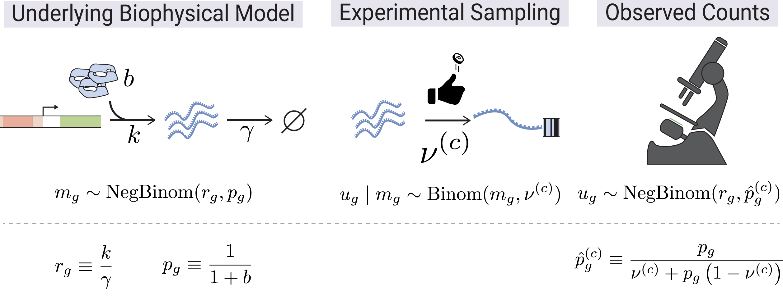
SCRIBE is grounded in a biophysical generative model of scRNA-seq count data. Transcription (rate \(b\)) and degradation (rate \(\gamma\)) set the steady-state mRNA content per gene, giving rise to a Negative Binomial distribution over true molecular counts \(m_g\) with parameters \(r_g\) and \(p_g\). During library preparation each molecule is independently captured with cell-specific probability \(\nu^{(c)}\), so the observed UMI count \(u_g\) follows a Binomial sub-sampling of \(m_g\). Marginalizing over the latent counts yields a Negative Binomial likelihood for the observations with an effective success probability \(\hat{p}_g^{(c)}\) that absorbs the capture efficiency.

For the full mathematical derivation, see the Theory section.

Why SCRIBE?

• Unified Framework: Single scribe.fit() interface for SVI, MCMC, and VAE inference methods
• Compositional Models: Four constructive likelihoods -- from the base Negative Binomial up to zero-inflated models with variable capture probability
• Compositional Differential Expression: Bayesian DE in log-ratio coordinates with proper uncertainty propagation and error control (lfsr, PEFP)
• Model Comparison: WAIC, PSIS-LOO, stacking weights, and goodness-of-fit diagnostics for principled model selection
• GPU Accelerated: JAX-based implementation with automatic GPU support
• Flexible Architecture: Three parameterizations, constrained/unconstrained modes, hierarchical priors, horseshoe sparsity, and normalizing flows
• Scalable: From small experiments to large-scale atlases with mini-batch support
• Production-Ready CLI: scribe-infer provides reproducible, config-driven inference with SLURM integration and automatic covariate-split orchestration; scribe-visualize generates diagnostic plots for any completed run

Key Features

• Three Inference Methods:
  • SVI for speed and scalability
  • MCMC (NUTS) for exact Bayesian inference
  • VAE for representation learning with normalizing flow priors
• Constructive Likelihood System: Negative Binomial as the base, extended with zero inflation and/or variable capture probability
• Multiple Parameterizations: Canonical, mean probs, and mean odds (with linked / odds_ratio aliases), constrained or unconstrained priors
• Advanced Guide Families: Mean-field, low-rank, joint low-rank, and amortized variational guides
• Mixture Models: K-component mixtures for cell type discovery with annotation-guided priors
• Hierarchical Priors: Gene-specific and dataset-level hierarchical structures with optional horseshoe sparsity
• Bayesian Differential Expression: Parametric, empirical (Monte Carlo), and shrinkage (empirical Bayes) methods in CLR/ILR coordinates
• Model Comparison: WAIC, PSIS-LOO, stacking, per-gene elpd, and goodness-of-fit via randomized quantile residuals
• Seamless Integration: Works with AnnData and the scanpy ecosystem

Model Construction Space

SCRIBE models are built compositionally. The likelihood is constructed by layering extensions on top of a base Negative Binomial (NB) model, then configured with a parameterization, constraint mode, optional extensions, and an inference method:

%%{init: {'theme': 'base', 'themeVariables': {'primaryColor': '#dce5f1', 'primaryTextColor': '#231f20', 'primaryBorderColor': '#4f7cbb', 'lineColor': '#272C68', 'secondaryColor': '#f0e8f4', 'tertiaryColor': '#ccf1e5'}}}%%
graph TD
    subgraph likelihood ["1 - Likelihood Construction"]
        NB["Negative Binomial<br/><i>base model</i>"]
        ZINB["Zero-Inflated NB"]
        NBcapture["NB + variable capture"]
        ZINBcapture["ZINB + variable capture"]
        NB -->|"+ zero inflation"| ZINB
        NB -->|"+ variable capture"| NBcapture
        ZINB -->|"+ variable capture"| ZINBcapture
        NBcapture -->|"+ zero inflation"| ZINBcapture
    end

    subgraph parameterization ["2 - Parameterization"]
        canonical["canonical<br/><i>sample p, r directly</i>"]
        meanProbs["mean_prob<br/><i>sample p, mu; derive r</i>"]
        meanOdds["mean_odds<br/><i>sample phi, mu; derive p, r</i>"]
    end

    subgraph constraint ["3 - Constraint Mode"]
        constrained["constrained<br/><i>Beta, LogNormal, BetaPrime</i>"]
        unconstr["unconstrained<br/><i>Normal + transforms</i>"]
    end

    subgraph extensions ["4 - Optional Extensions"]
        mixture["Mixture<br/><i>K components</i>"]
        hierarchical["Hierarchical Priors<br/><i>gene-specific p, gate</i>"]
        multiDataset["Multi-Dataset<br/><i>per-dataset parameters</i>"]
        horseshoe["Horseshoe<br/><i>sparsity priors</i>"]
        annotationPrior["Annotation Priors<br/><i>soft cell-type labels</i>"]
        bioCap["Biology-Informed<br/><i>capture prior</i>"]
    end

    subgraph infer ["5 - Inference Method"]
        SVI_node["SVI<br/><i>fast, scalable</i>"]
        MCMC_node["MCMC<br/><i>exact posterior</i>"]
        VAE_node["VAE<br/><i>learned representations</i>"]
    end

    subgraph guide ["6 - Guide Family"]
        meanField["Mean-Field"]
        lowRank["Low-Rank"]
        jointLowRank["Joint Low-Rank"]
        amortized["Amortized"]
        flows["Normalizing Flows<br/><i>VAE prior</i>"]
    end

    likelihood --> parameterization
    parameterization --> constraint
    constraint --> extensions
    extensions --> infer
    SVI_node --> guide
    VAE_node --> guide

    %% Brand color styling for subgraphs
    style likelihood fill:#ccf1e5,stroke:#00b97c,stroke-width:2px
    style parameterization fill:#dce5f1,stroke:#4f7cbb,stroke-width:2px
    style constraint fill:#f0e8f4,stroke:#b48ec6,stroke-width:2px
    style extensions fill:#fcf1ce,stroke:#ebb800,stroke-width:2px
    style infer fill:#e3e5fc,stroke:#767eed,stroke-width:2px
    style guide fill:#effbfa,stroke:#28898A,stroke-width:2px

This compositional design means you can combine 4 likelihoods x 3 parameterizations x 2 constraint modes as a starting point, then layer on mixture components, hierarchical priors, multi-dataset structure, and more.

Available Models

NB family

SCRIBE's NB-family likelihoods build on each other -- the base Negative Binomial can be extended with zero inflation and/or variable capture probability:

Likelihood	Code	Construction	Extra Parameters	Best For
Negative Binomial	"nbdm"	Base model	--	Very tight total-UMI distribution
NB + variable capture	"nbvcp"	NB + capture probability	p_capture	Typical heterogeneous library sizes
Zero-Inflated NB	"zinb"	NB + zero inflation	gate	Excess zeros after VCP ruled out
ZINB + variable capture	"zinbvcp"	ZINB + capture probability	gate, p_capture	Both ZI and VCP supported by diagnostics

Any of these can be extended to mixture models with n_components=K for subpopulation analysis.

Logistic-Normal Multinomial (LNM) family

LNM extends the NB family with a VAE-decoded compositional structure in additive log-ratio (ALR) coordinates. Counts factor into total counts (NB) and composition (Multinomial), with gene-gene correlations captured by a low-rank Gaussian in ALR space.

Likelihood	Code	Construction	When to Use
LNM	"lnm"	NB totals + VAE	Compositional inference + DE
LNM + variable capture	"lnmvcp"	LNM + capture prob	LNM with variable sequencing depth

See Logistic-Normal Multinomial for the theory.

Poisson-LogNormal (PLN) and NB-LogNormal (NBLN) families

PLN and NBLN parameterize gene-gene covariance directly through a low-rank log-normal latent on the gene rates (Σ = WW^⊤ + diag(d)). PLN uses a Poisson observation channel; NBLN uses NB with per-gene dispersion r_g. Both fit via a Laplace-EM workflow with optional SVI-cascade warm-start.

Likelihood	Code	Construction	When to Use
PLN	"pln"	Poisson + low-rank LN	Absolute counts with explicit gene-gene covariance
NBLN	"nbln"	NB + low-rank LN	PLN + per-gene overdispersion (the typical scRNA-seq case)

See Poisson-LogNormal, NB-LogNormal, and Loadings shrinkage.

Two-state promoter (Poisson-Beta) family

The two-state promoter likelihood is a Poisson-Beta compound: p_gc ~ Beta(α_g, β_g) and u_gc | p_gc ~ Poisson(r̂_g · p_gc · ν_c) with p_gc independent per (gene, cell). It captures the bursty / bimodal genes the NB family cannot fit. The closed-form NB is recovered in the k_off → ∞ limit, so the two-state model nests inside the NB family rather than competing with it. The marginal log-likelihood is evaluated via fixed Gauss-Legendre quadrature over p.

Likelihood	Code	Construction	When to Use
TwoState	"twostate"	Poisson-Beta compound	Bursty / bimodal genes the NB cannot fit
TwoState + var capture	"twostatevcp"	TwoState + capture prob	Bursty genes with variable sequencing depth

The TwoState family ships with four parameterizations of its shape coordinate — two_state_natural, two_state_ratio, two_state_mean_fano, two_state_moment_delta. All four support mixture models (n_components=K) via the same API as the NB family and both constrained (LogNormalSpec, BetaSpec) and unconstrained (Normal + transform) guides. Under unconstrained=True, the default positive_transform is {"mu": "exp"} (multiplicative-step geometry for gene means that span orders of magnitude). See Two-state promoter for the full math and a decision guide.

Parameterizations

NB-family likelihoods (nbdm / zinb / nbvcp / zinbvcp) accept three parameterizations of the dispersion/mean structure:

Name	parameterization=	Aliases	Core	Derived	When to Use
Canonical	canonical	standard	p, r	--	Direct interpretation
Mean probs	mean_prob	linked	p, mu	r = mu(1-p)/p	Couples mean and p
Mean odds	mean_odds	odds_ratio	phi, mu	p = 1/(1+phi), r = mu*phi	Stable when p is near 1

TwoState-family likelihoods (twostate / twostatevcp) accept four parameterizations of their shape coordinate — see the Two-state promoter theory page. PLN, NBLN, LNM, and LNMVCP use decoder-based parameterizations auto-selected by the factory; the parameterization argument is not exposed for those families.

Constrained vs Unconstrained

Mode	Prior Distributions	Use Case
Constrained	Beta, LogNormal, BetaPrime	Default; interpretable parameters
Unconstrained	Normal + sigmoid/exp transforms	Optimization-friendly; required for hierarchical priors

Quick Start

import scribe
import scanpy as sc

# Load your single-cell data
adata = sc.read_h5ad("your_data.h5ad")

# Default model includes variable capture; add low-rank guide for gene-gene correlations
results = scribe.fit(adata, guide_rank=64)

# Analyze results
posterior_samples = results.get_posterior_samples()

Customize with Simple Arguments

# Zero-inflated model with more optimization steps
results = scribe.fit(
    adata,
    zero_inflation=True,
    n_steps=100_000,
    batch_size=512,
)

# Linked parameterization with low-rank guide
results = scribe.fit(
    adata,
    model="nbdm",
    parameterization="linked",
    guide_rank=15,
)

# Mixture model for cell type discovery
results = scribe.fit(
    adata,
    zero_inflation=True,
    n_components=3,
    n_steps=150_000,
)

Choose Your Inference Method

Method	Engine	Precision	Use Case
SVI	Adam optimizer	float32	Fast exploration, large datasets
MCMC	NUTS sampler	float64	Exact posterior, gold standard
VAE	Encoder-decoder	float32	Latent representations, embeddings

# Fast exploration with SVI (default)
svi_results = scribe.fit(adata, zero_inflation=True, n_steps=75_000)

# Exact inference with MCMC
mcmc_results = scribe.fit(
    adata,
    model="nbdm",
    inference_method="mcmc",
    n_samples=3000,
    n_chains=4,
)

# Representation learning with VAE
vae_results = scribe.fit(
    adata,
    model="nbdm",
    inference_method="vae",
    n_steps=50_000,
)

Differential Expression

SCRIBE provides a fully Bayesian differential expression framework that respects the compositional nature of scRNA-seq data. All comparisons are performed in log-ratio coordinates (CLR/ILR), propagating full posterior uncertainty.

Method	Description	Use Case
Parametric	Analytic Gaussian in ALR space	Fast, requires low-rank logistic-normal fit
Empirical	Monte Carlo CLR differences	Assumption-free, from posterior samples
Shrinkage	Empirical Bayes scale-mixture prior	Improved per-gene inference, borrows strength across genes

import jax.numpy as jnp
from scribe import compare

# Fit two conditions (default likelihood; 3-component mixture)
results_ctrl = scribe.fit(adata_ctrl, n_components=3)
results_treat = scribe.fit(adata_treat, n_components=3)

# Empirical DE between component 0 across conditions
de = compare(
    results_treat, results_ctrl,
    method="empirical",
    component_A=0, component_B=0,
)

# Gene-level results with practical significance threshold
gene_results = de.gene_level(tau=jnp.log(1.1))

# Call DE genes controlling false sign rate
is_de = de.call_genes(lfsr_threshold=0.05)

Full guide: Differential Expression

Model Comparison

Principled Bayesian model comparison with WAIC, PSIS-LOO, stacking weights, per-gene elpd differences, and goodness-of-fit diagnostics:

from scribe import compare_models

mc = compare_models(
    [results_nb, results_hierarchical],
    counts=counts,
    model_names=["NB", "Hierarchical"],
    gene_names=gene_names,
)

# Ranked comparison table
print(mc.summary())

# Per-gene elpd differences
gene_df = mc.gene_level_comparison("NB", "Hierarchical")

Full guide: Model Comparison

Getting Started

• Installation

  ---

  Install SCRIBE and set up your environment

  Installation guide

• Quick Overview

  ---

  Understand the probabilistic approach behind SCRIBE

  Quick overview

• Quickstart

  ---

  Run your first inference in minutes

  Quickstart tutorial

• Theory

  ---

  Mathematical foundations of the SCRIBE models

  Theory

• Model Selection

  ---

  Choose the right model for your data

  Model Selection

• User Guide

  ---

  Inference methods, DE, model comparison, and more

  User guide

• scribe-infer CLI

  ---

  Reproducible, config-driven inference with SLURM integration

  CLI guide

• scribe-visualize CLI

  ---

  Post-inference diagnostic plots with recursive and SLURM support

  Visualization guide

• API Reference

  ---

  Full reference for all modules and classes

  API reference